The twisted history of political mapping
We live in what is endlessly described as an era of unprecedented partisanship, with Americans polarized into red and blue camps and no convergence in sight. But much of the nation’s history was characterized by intense political rivalry, especially the late nineteenth century.
In 1876 the United States celebrated its centennial in the midst of a terrible depression sparked by the Panic of 1873. In some cities unemployment reached 25 percent, casting a significant pall over the celebration mounted in Philadelphia that spring. The mood worsened after the November presidential elections, which left Democrat Samuel Tilden in an electoral tie with Republican Rutherford Hayes. The atmosphere was chaotic, with accusations of voter suppression, rigged ballots, questionable returns, and eleventh-hour statehood for Colorado, which threw three crucial electoral votes to Hayes. The election was ultimately decided by a committee, which gave Republicans ongoing control of the White House. In return the party agreed to pull the remaining troops out of the South, thereby ending Reconstruction.
This “Great Compromise” came during one of the most partisan periods in American history, and much of the staunch party loyalties had been forged in the recent Civil War. White Southerners were committed in their resistance to the Republicans for years after Appomattox, and by 1876 had coalesced into a block of unquestioned support for the Democratic Party that would last well into the twentieth century. In response, Republicans repeatedly “waved the bloody shirt” to remind Americans that it was they—the party of Lincoln—that had preserved the Union through the late war.
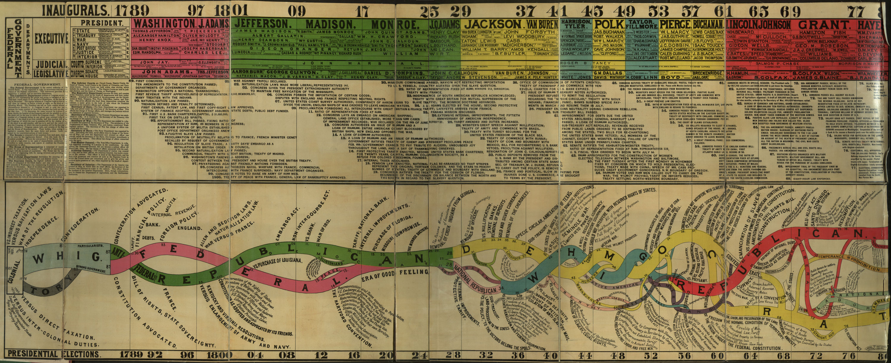
The riveting and decidedly partisan centennial election also coincided with the emergence of politics as a field of academic study. At its outset, “political science” focused on the evolution of American democracy and party behavior. This heightened interest in the nation’s political history prompted a slew of charts, maps, and graphs designed to make sense of the past “century of progress.” Among the most fascinating of these was Walter Houghton’s huge, elaborate chart of U.S. political history. A Midwestern educator, Houghton touted this as a “compass” to guide Americans through their complex political past.
Click to open in new window.
At first glance the chart is disorienting, but it has its own internal logic. The top half is a straightforward timeline of elected leaders, important events, and landmark legislation rendered in ridiculously small type. It’s in the lower half where Houghton tried to find patterns in that chronology. He assigned a line to every party in electoral history, then measured the popular support for the party with comparatively thicker or thinner lines. The party occupying the White House is always placed on top.
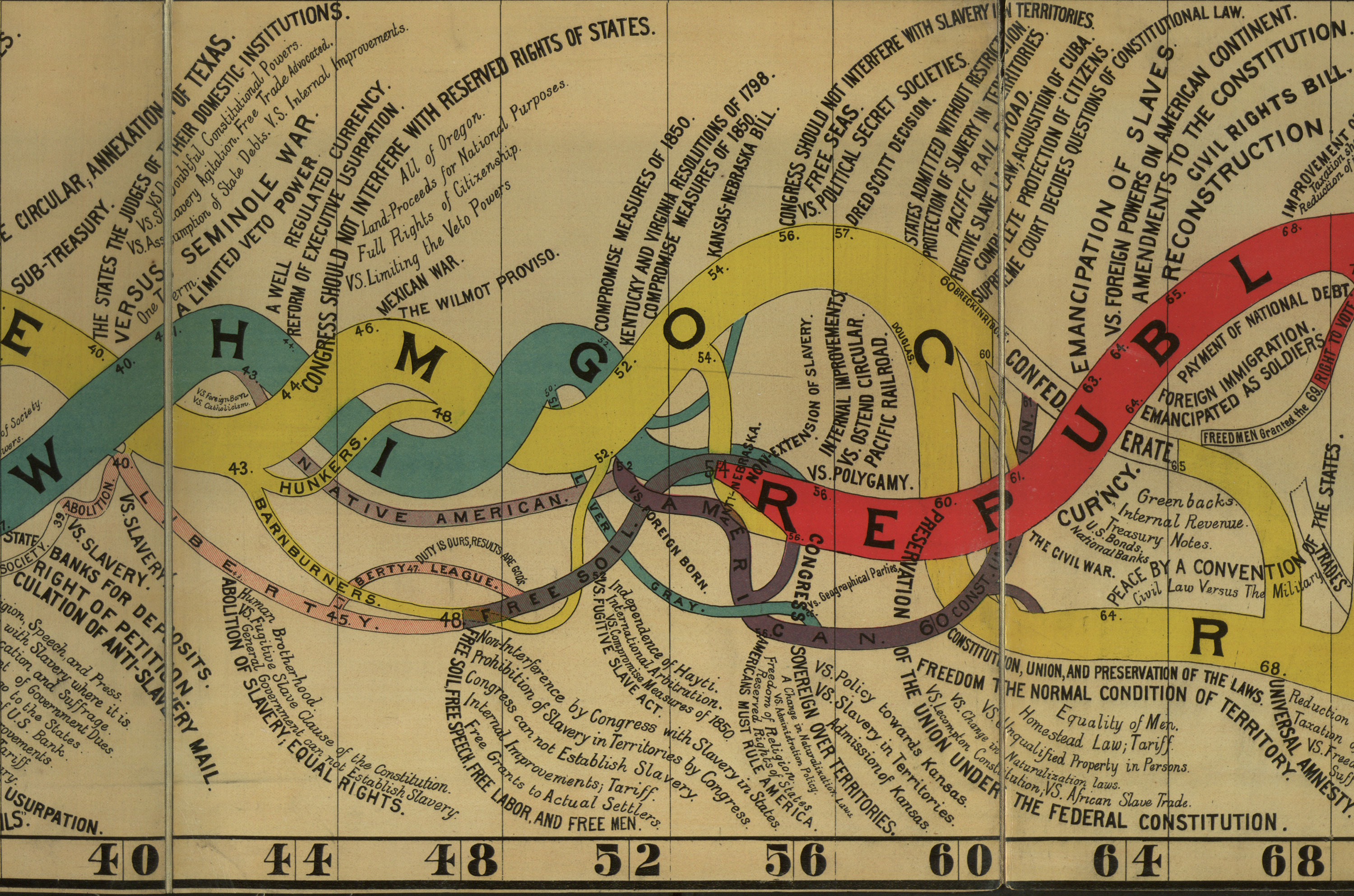
The detail below captures the run up to the Civil War, when the decline of the Whigs and the erosion of the Democrats created a vacuum filled by a new Republican party, devoted to halting the extension of slavery into the territories.
Click to open in new window.
Houghton’s “conspectus” of political history caught on, and was copied and updated through the end of the century. Like so many other timelines and charts made to commemorate the nation’s centennial, it resonated with readers as an attempt to see some order—or at least form—in the chaos of history.
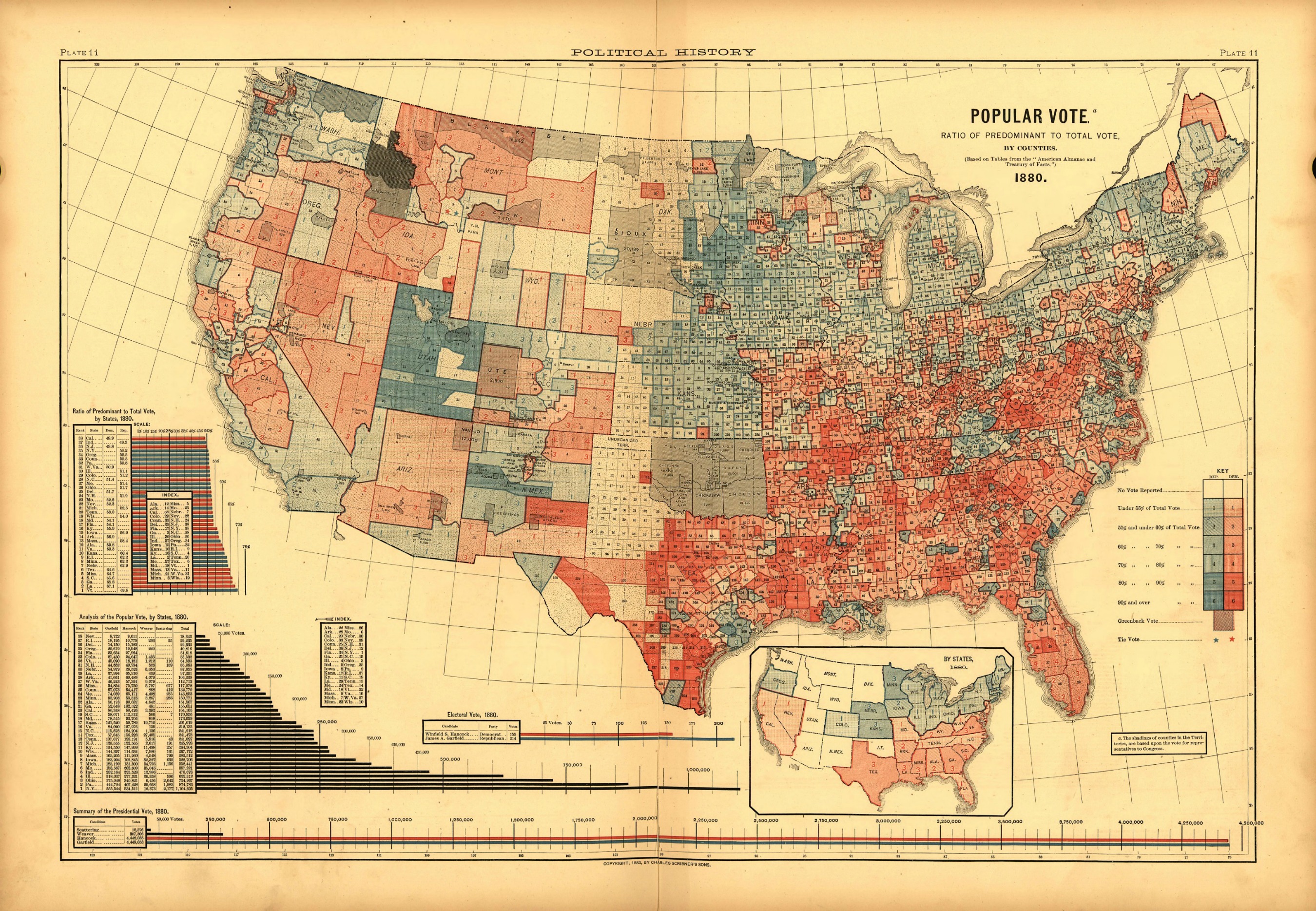
At the same time that Houghton was charting the evolution of political behavior, the Census Office released an ambitious effort to map the nation’s electoral history. In 1883, Census Superintendent Henry Gannett published the massive Scribner’s Statistical Atlas, which included maps of each presidential election. The series ended with an unprecedented attempt to map the returns of the 1880 presidential election not just at the state but the county level.
Click to open in new window.
Such data maps are routine today. But this one stunned nineteenth-century Americans by showing them a nation organized not according to railroads and town, or mountains and rivers, but Democrats and Republicans. The parties, of course, represented entirely different agendas then, and even their color associations were reversed. On the Scribner map, red denotes Democrats, while blue marks Republicans. Yet the overall portrait is strangely familiar, with red blanketing much of the south while blue spreads across the north. (As to the color scheme reversal, it’s a bit of a mystery. Republicans are now generally represented with red and Democrats with blue, a change that seems to have taken hold sometime after the 2000 election. But other colors were used as well through the twentieth century, as in Paullin and Wright’s Atlas of 1932.)
The 1880 campaign itself was rather routine, with little of substance to differentiate the two parties aside from their positions on tariff policy. Yet the election itself was as much of a nail biter as 1876 had been: nine million Americans turned out, and when it was over Republican James Garfield had outpolled the Democrat by a margin of just 7,000 votes nationwide.
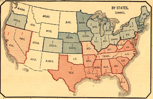
Focus on the outcome by states—the only measure that matters in the Electoral College—and the map shows a nation that seems hopelessly divided along a north-south axis, still fighting the Civil War by other means. Democrats control the former slave states, while Republicans hold an edge in the northeast and Midwest, as the inset captures.
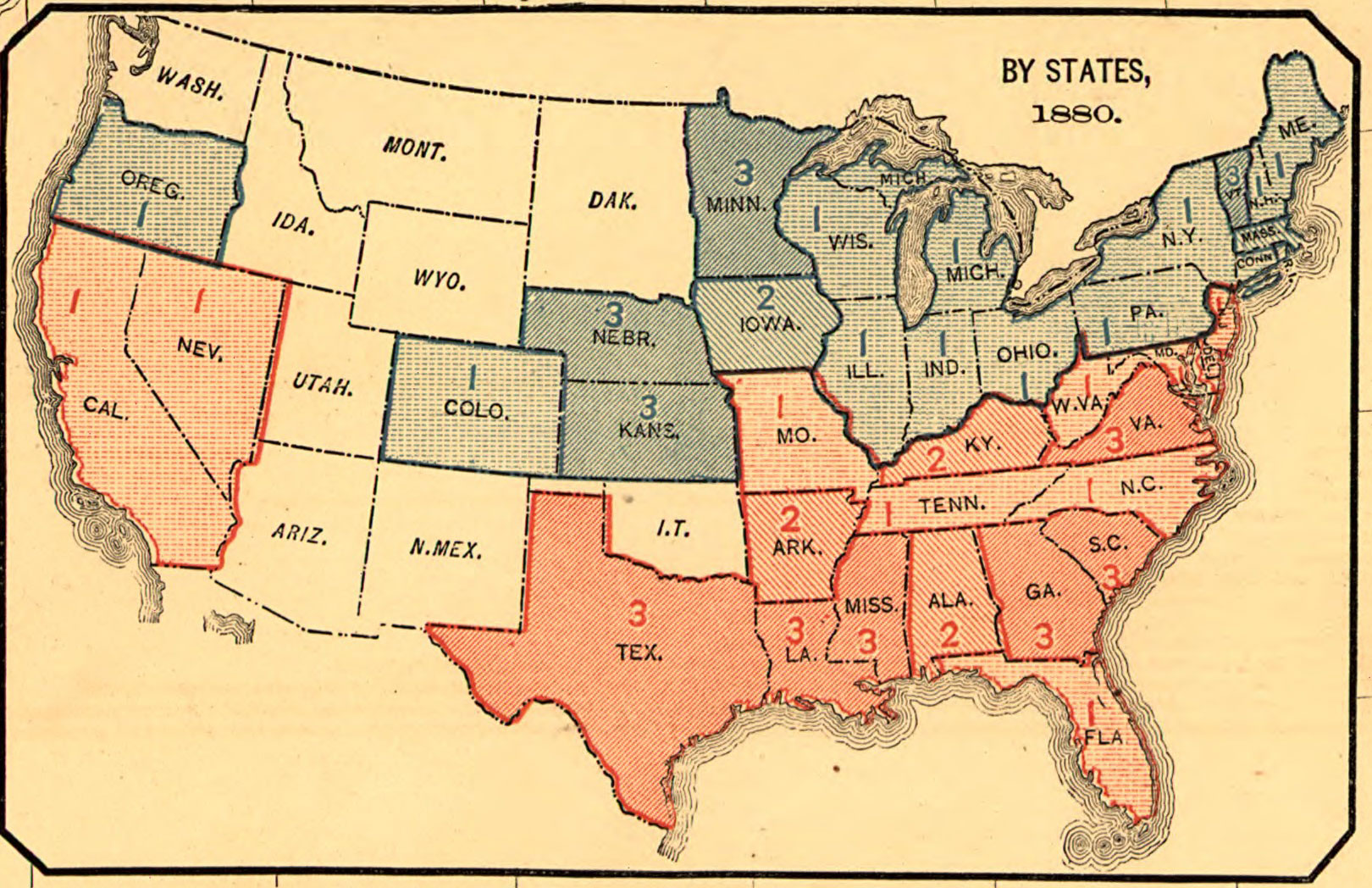
And in a move that would have impressed Nate Silver, Superintendent Gannett ranked each of these states according to the decisiveness of party victory, from least to most partisan.
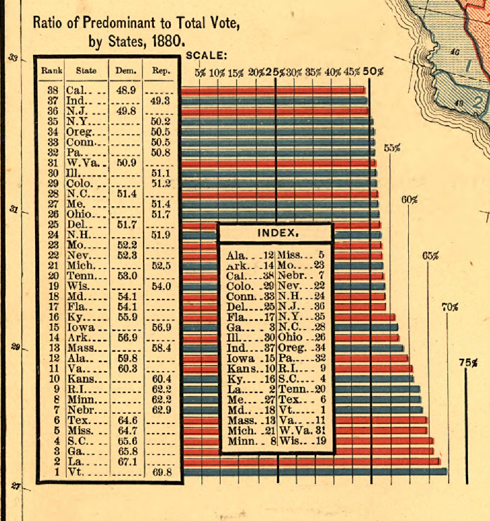
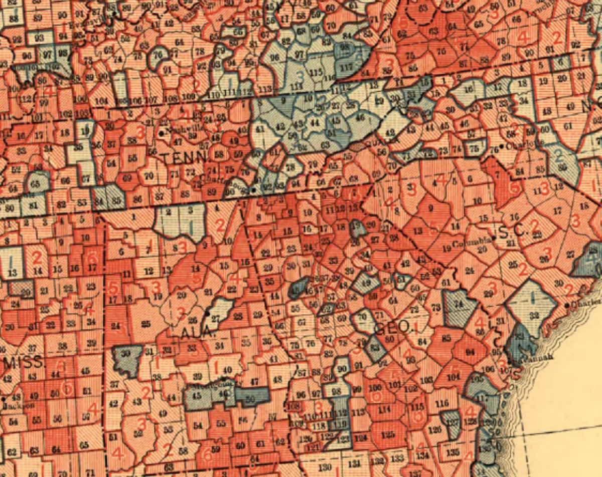
But Gannett realized that though the state outcomes determined the presidential election, a far more nuanced picture of voter behavior could be captured at the county level. For this reason he relegated the Electoral College map to an inset in order to feature a much larger map of county outcomes. Take a look again at the larger map, and notice the variation. Though the “solid south” had already materialized, a few pockets of support for Garfield endured, as in eastern Tennessee, where anti-Confederate sentiment during the Civil War translated into Republican counties thereafter. Further south, blacks enfranchised by the Fifteenth Amendment created a few small Republican strongholds along the cotton belt, though these disappeared once the black vote was effectively suppressed by poll taxes and other tools. Across the country, the map showed just how much variation the Electoral College concealed.
Click to open in new window.
Then Gannett went even further with his geovisual adventure: it was not enough just to sort the nation into red and blue counties, so he designed a scale of shade to measure not just victory but depth of victory. In any given county one could see not just who won, but how handily.
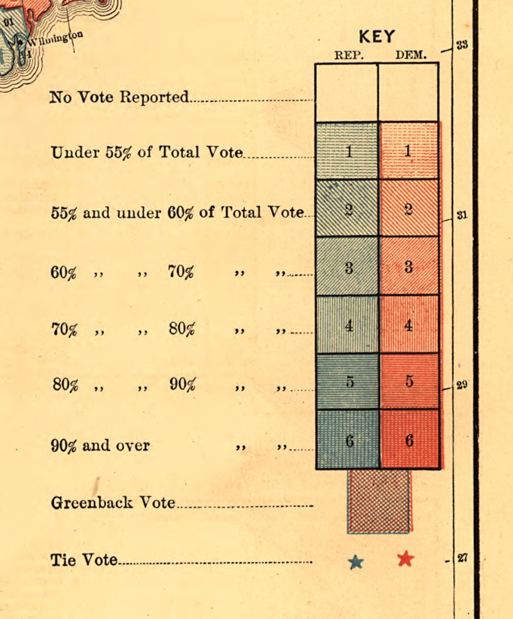
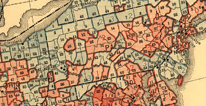
The light pink areas of the upper south indicated that while the Democrats had prevailed, their control was relatively weak. Conversely, light blue areas throughout the northeast—such as in Pennsylvania below—indicated a Republican party struggling to maintain its hold over regions of massive immigration, industrial turmoil, and growing class conflict. In fact, even though Garfield easily won the Electoral College, the switch of just a few thousand votes in New York would have changed the outcome.
Click to open in new window.
The map may not look advanced today, but in 1883 it broke new ground by enabling Americans to visualize the spatial dynamics of political power. Readers responded enthusiastically. One reviewer pointed to the Republican counties in Arkansas—something left invisible on a map of the Electoral College returns—and wondered what other oddities of geography and history might be uncovered when election returns were more systematically measured. In other words, the map revealed spatial patterns and relationships that might otherwise remain hidden, or only known anecdotally. Perhaps its no coincidence that at the same time the two parties began to launch more coordinated, disciplined, nationwide campaigns, creating a system of two-party rule that we have lived with ever since.
Houghton conspectus courtesy University of Denver; map of 1880 election courtesy Library of Congress.
Use controls to zoom and pan.